Complexity
- Imagine you're a chef in a restaurant, and you have a recipe to cook a dish. The complexity of the recipe can be thought of as how much time and effort it takes to make the dish based on the number of ingredients and steps involved.
- In computer science, complexity refers to how much time (or sometimes memory) a program or algorithm takes to run, based on the size of the input. This is important because we want programs to be efficient, just like you'd want your cooking process to be efficient in the kitchen.
Some complexity metrics:
Metric | Description |
|---|---|
| Cyclomatic complexity (CC) | Measures the number of linearly independent paths through a program's source code. |
| Halstead complexity measures (HCM) | Measures the size and difficulty of understanding a program's source code. |
| Maintainability index (MI) | Measures the maintainability of a program. |
| Lines of code (LOC) | Measures the size of a program in terms of the number of lines of code. |
| Function points (FP) | Measures the size of a program in terms of its functionality. |
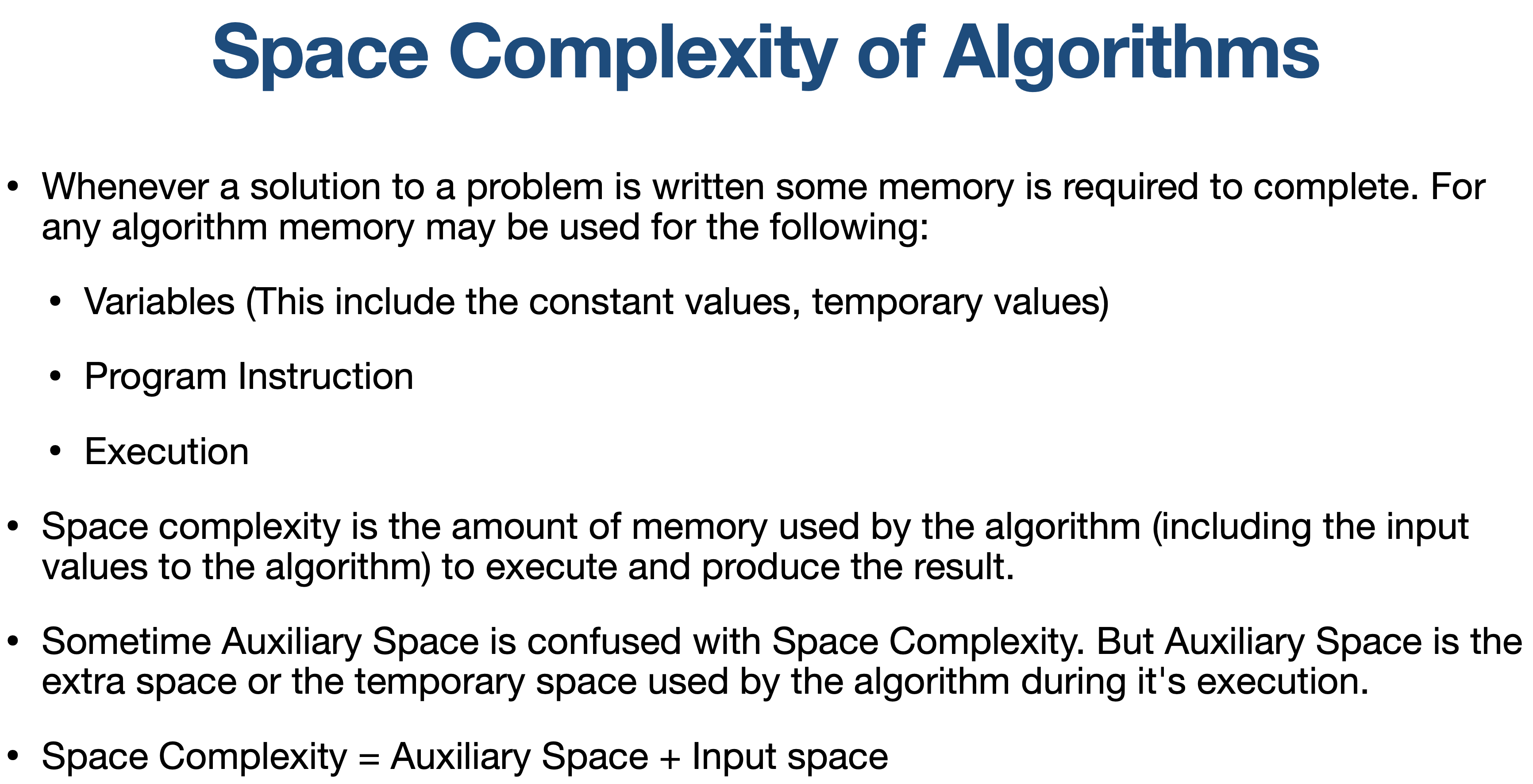
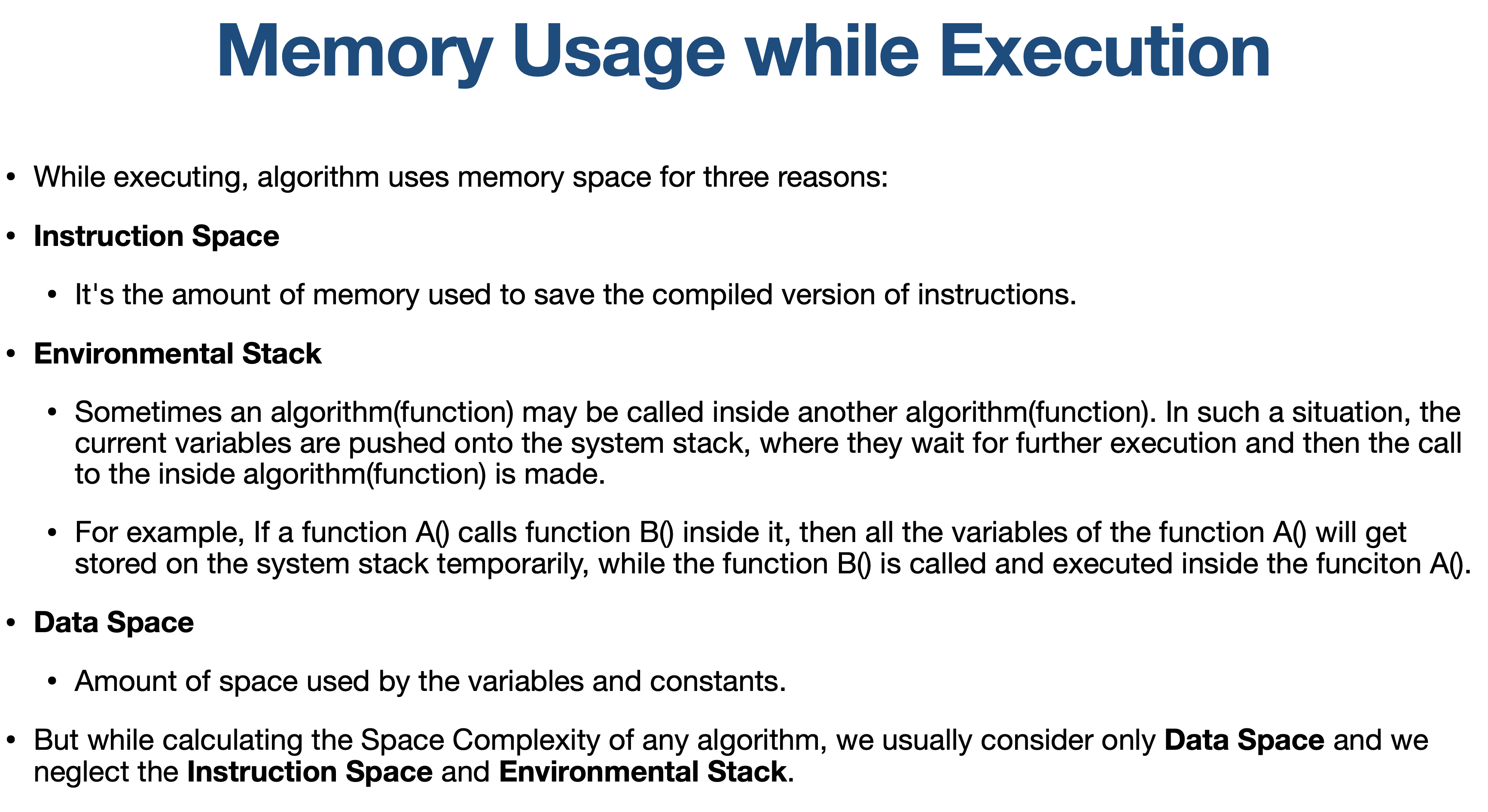
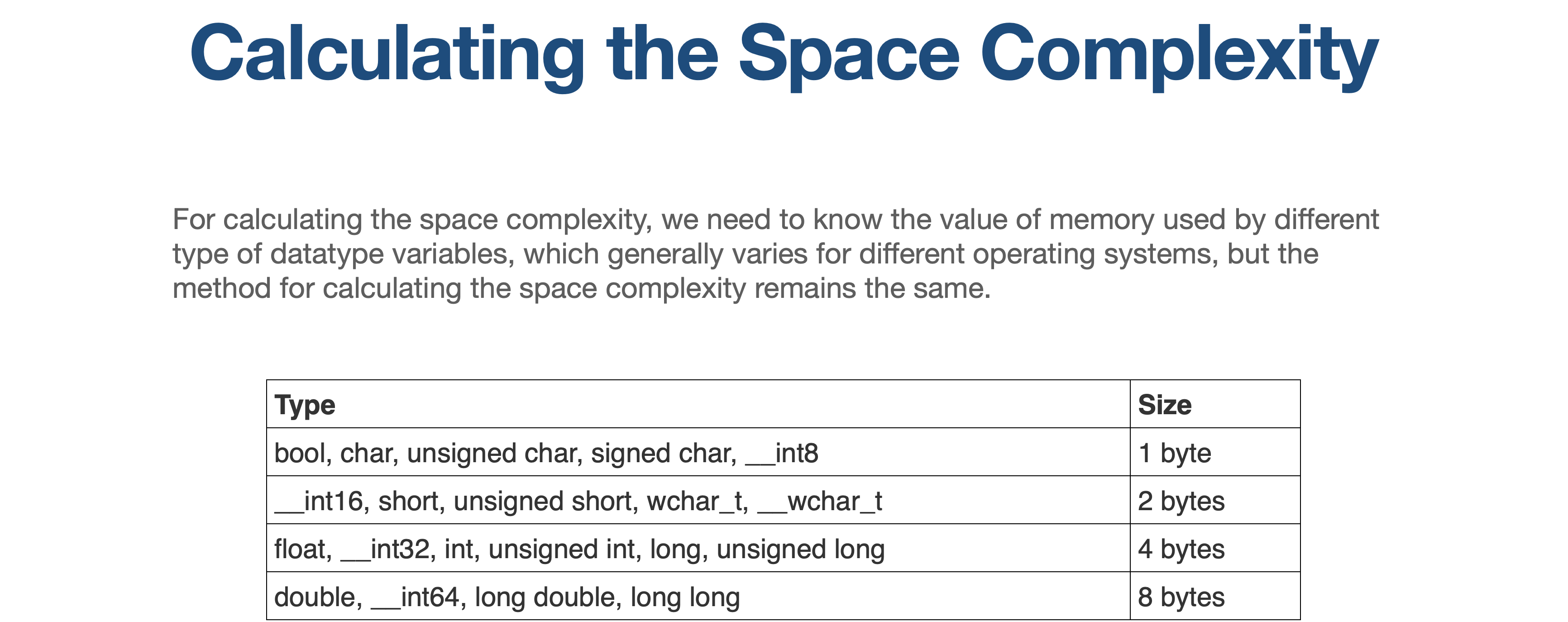
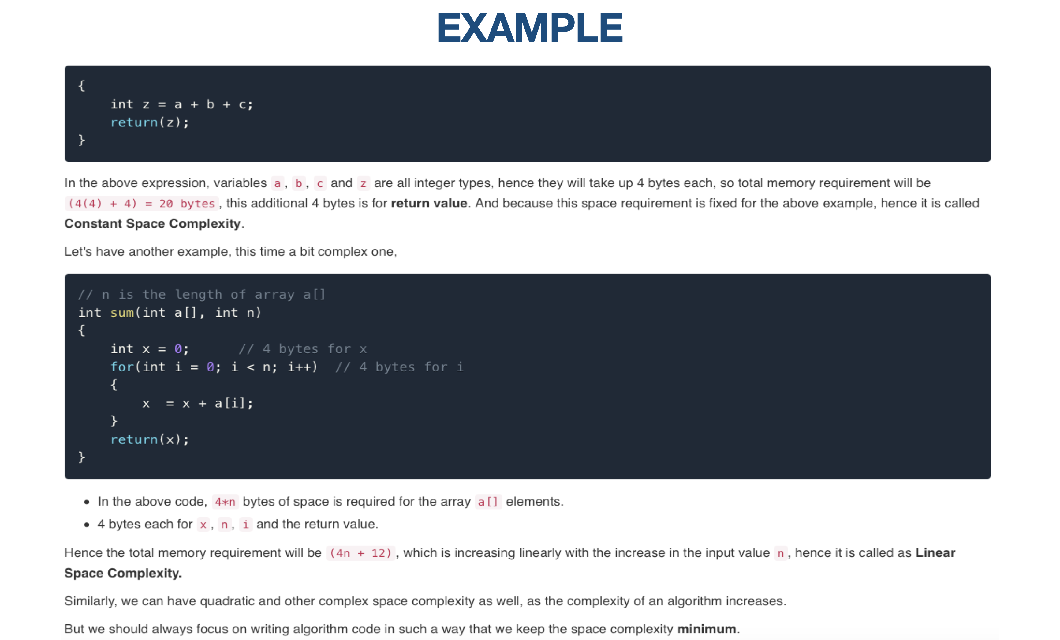
There are two main types of complexity: time complexity and space complexity.
Time Complexity
Time complexity measures how many operations an algorithm takes as the size of the input grows. It's like measuring how long it takes to cook a dish when the recipe gets more complex.
The time complexity of algorithms is most commonly expressed using the big O notation. It's an asymptotic notation to represent the time complexity.
Time Complexity is most commonly estimated by counting the number of elementary steps performed by any algorithm to finish execution.
Big O Notation
Big O notation is a way of describing how the running time of an algorithm grows as the input size grows. It is a mathematical way of saying that the running time of an algorithm is asymptotically equal to some function of the input size.
In simple English, big O notation can be thought of as the worst-case running time of an algorithm. It is the upper bound on the running time of the algorithm, no matter what the input data is.
The most common big O notations are:
- O(1): Constant time. The running time does not depend on the input size.
- O(log n): Logarithmic time. The running time grows logarithmically with the input size.
- O(n): Linear time. The running time grows linearly with the input size.
- O(n log n): Logarithmic-linear time. The running time grows logarithmically with the input size, but the constant factor is higher than for O(log n).
- O(n^2): Quadratic time. The running time grows quadratically with the input size.
- O(2^n): Exponential time. The running time grows exponentially with the input size.
O(1)
An algorithm with O(1) time complexity takes the same amount of time regardless of the input size. It's like grabbing an item from a well-organized fridge – it doesn't matter how many items are inside; you can find what you need quickly.
def get_first_element(lst):
    return lst[0]
In this example, the get_first_element function takes a list lst as input and immediately returns the first element of the list using indexing. It doesn't matter how large the list is; the function always takes the same amount of time because it directly accesses the first element using a fixed operation (indexing by 0).
No matter how big the list gets, the time taken to retrieve the first element remains constant. This is why the time complexity of this function is O(1), indicating that its runtime doesn't depend on the input size.
O(n)
An algorithm with O(n) time complexity means that the time taken grows linearly with the input size. It's like counting items in a grocery bag; each item takes a constant amount of time.
Example: Eating chips out of a bag, one at a time. If there are n chips in the bag, you need to dip your hand in the bag, take a chip out and put it in your mouth n times. Thus the linear complexity.
def find_element(lst, target):
    for i, element in enumerate(lst):
        if element == target:
            return i
    return -1
In this example, the find_element function takes a list lst and a target value as inputs. It then iterates through the list using a loop and checks each element to see if it matches the target value. If a match is found, the index of the matching element is returned. If no match is found, it returns -1.
The time taken by this function is directly proportional to the size of the list. As the list grows larger, the loop has to iterate through more elements to find the target value. This linear relationship between the input size and the time taken gives this function an O(n) time complexity.
O(n^2)
An algorithm with O(n^2) time complexity means that the time taken is proportional to the square of the input size. It's like comparing every pair of items in a list.
def quadratic_algo(items):
    for item in items:
        for item2 in items:
            print(item, ' ' ,item2)

quadratic_algo([4, 5, 6, 8])
We have an outer loop that iterates through all the items in the input list and then a nested inner loop, which again iterates through all the items in the input list. The total number of steps performed is n*n, where n is the number of items in the input array.
O(log n)
Say, you want to cut a pizza in 8 equal slices. To get the first slice out, you need to cut the pizza only 3 () times. You first slice the pizza into 2 pieces, then you cut each slice into 2 more pieces and so on. Hence the complexity of O(log n).
An algorithm with O(log n) time complexity means that as the input size grows, the time taken increases but at a slow rate.
def binary_search(sorted_lst, target):
    left, right = 0, len(sorted_lst) - 1
    while left <= right:
        mid = (left + right) // 2
        if sorted_lst[mid] == target:
            return mid
        elif sorted_lst[mid] < target:
            left = mid + 1
        else:
            right = mid - 1
    return -1
In this example, the binary_search function takes a sorted list sorted_lst and a target value as inputs. It performs a binary search to find the index of the target value within the list.
The binary search algorithm repeatedly divides the search range in half, discarding half of the remaining elements each time. This efficient "divide and conquer" approach results in a logarithmic growth rate. As the input size (length of the list) increases, the number of iterations required to find the target value only increases slowly, following a logarithmic pattern.
This logarithmic relationship between the input size and the number of operations gives the binary_search function an O(log n) time complexity.
O(2^n)
def recursive_fibonacci(n):
    if n <= 1:
        return n
    else:
        return recursive_fibonacci(n - 1) + recursive_fibonacci(n - 2)

for i in range(1,10):
    print(recursive_fibonacci(i))
In this example, the recursive_fibonacci function calculates the Fibonacci number at index n using a recursive approach. It uses the definition of the Fibonacci sequence, where each number is the sum of the two preceding ones.
However, the way this function is implemented leads to an exponential growth in the number of recursive calls. For each recursive call, two more calls are made: one for n - 1 and one for n - 2. This results in an exponential increase in the number of function calls and computations.
As a result, the time complexity of this function is O(2^n). The number of operations doubles with each increase in n, leading to an exponential growth in time complexity. This makes the function highly inefficient for larger values of n, as the number of computations grows rapidly.
The below table indicates the number of recursive calls per input series. As you can see at each step the operational complexity increases almost exponentially.